So today I am giving a talk in the Subfactor seminar here at Berkeley, and I thought it might by nice to write my pre-talk notes here on the blog, rather then on pieces of paper destined for the recycling bin.
This talk is about how you can use Planar algebras planar techniques to construct 3D topological quantum field theories (TQFTs) and is supposed to be introductory. We’ve discussed planar algebras on this blog here and here.
So the first order of buisness: What is a TQFT?
According to the Atyiah-Segal axioms a TQFT is a functor.
Specifically a TQFT is a functor from a bordism category of manifolds to the category of vector spaces. This bordism category has a dimension D associated to it, and so we get D-dimensional TQFTs. Sometimes these are called “N+1 TQFTs” where N+1 = D. Thus a 1+1 TQFT is really 2-dimensional and a 2+1 TQFT is 3-dimensional. I swear this is just a notation and not because we can’t add.
There are a couple variations on the bordism category that people consider depending on what bells and whistles they want to add to their manifolds. Our bells and whistles will be orientations. For us, the bordism category of dimension D will be the following:
- Objects: Closed oriented (D-1)-manifolds.
- Morphisms: A morphism from
to
is an Equivalence class of Triples
, where W is an oriented compact D-manifold with boundary,
and
are inclusions, such that
is a decomposition of
into disjoint submanifolds.
Two triples are equivalent if there is an orientation preserving diffeomorphism 
The case we are most interested in today are D= 2 and 3.
So a TQFT is a functor from this bordism category to the category of vector spaces. Thus it associates a vector space to each (D-1)-manifold and a linear map to each D-manifold.
Both the bordism category and the category of vector spaces have additional structure and a TQFT is required to respect this structure. Precisely, the disjoint union for manifolds and the tensor prodct for vector spaces make both categories into symmetric monoidal categories and a TQFT is required to be a symmetric monoidal functor. Thus a TQFT sends the disjoint union of manifolds to the tensor product of vector spaces.
Why do people care about TQFTs?
We’ll I like TQFTs because, as we’ll see, they relate algebra and topology in many interesting ways. But other people like TQFTs for other reasons. For 3D TQFTs, one of the most important parts of a TQFT is that they give invariants of 3-manifolds. In fact any TQFT can be thought of as giving invariants for any bordism, but lets look at some simple manifolds and bordisms.
Suppose we have a TQFT called Z. Thus we get vector spaces Z(M) for each (D-1)-manifold M. One of my favorite (D-1)-manifolds is the empty manifold 

What are the endomorphisms of
So what does the TQFT do to these? Well a TQFT will give us a map from K to K, which is also known as a “number”. So, for example, part of a 3D TQFT associates to each closed 3-manifold a number, and this number only depends on the isomorphism class of the 3-manifold. Thus for any 3D TQFT we get 3-manifold invariants. In fact, as we discussed before, it might be that these invariants distinguish all 3-manifolds. Exciting stuff.
In the rest of this talk due to time constraints, we will be focusing on this number, but the rest of the TQFT is there too, lurking in the background.
Okay, so how does any of this relate to planar algebras?
One way to relate them is that we can use planar algebras (i.e. 2-dimensional algebras) to construct 3D TQFTs. We’ll see how in a bit, but let’s start with the easier case of how “linear algebras” (i.e. 1-dimensional algberas) allow us to build 2D TQFTs.
It all rests on the following key facts:
- For 2- and 3-manifolds the classes of TOP, PL, and DIFF are all the same. This means that any 3-manifold has a triangulation and that these give the same PL structure.
- Pachner’s theorem: Two closed triangulated n-manifolds are PL-homeomorphic if and only if it is possible to move between their trinagulations using a sequence of Pachner moves.
In each dimension, the Pachner moves are a finite list of local moves which relate triangulations. For example in dimension 2 we have:


These two moves are called the 2-2 move and the 3-1 move, respectively. This suggests the following strategy for constructing TQFTs/manifold invariants:
- Given a manifold, choose a triangulation.
- Use some algebraic gadget, such as an algebra or a planar algebra, to associate a number to the triangulation.
- Show that this number is invariant under the Pachner moves.
- If step 3 fails, go back to step 2 and try again.
- Repeat.
This really just constructs the closed manifold sector, but with a little extra work we can get the rest of the TQFT too.
Now we make the following loose analogy:
2D Case:
- Algebras.
- *-algebras.
- Frobenius Algberas
- symmetric Frobenius algebras
3D Case:
- Monoidal Categories.
- Monoidal Categories with duals.
- Pivotal Categories/Planar algebras.
- sphereical categories/planar algebras.
[I might explain a little about this analogy if time permits. I’m going to assume the audience knows what a planar algebra is. A Frobenius algebra is finite dimensional, has a trace 
How to build a 2D TQFT out of a symmetric Frobenius algebra:
We start be taking our 2-manifold and triangulating it. We also order the vertices. This gives each edge and face an orientation. The orientation of the face may agree or disagree with orientation of the surface.
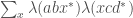
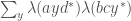
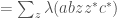
Next we choose a basis for the Frobenius algebra. The idea is that we are going to label the edges of the triangulation by elements of this basis. Given this labeling we are going to get a number for each triangle and we are going to multiply these numbers to get an overall number for the labeled triangulation. Summing over all possible labelings gives us a number for the triangulation, completing step 2 of our overall strategy.
So how are we going to get this number? Well a labeled simplex looks like this:

where a,b, and c are basis elements of our algebra. If the orientation agrees with our surface, what we can do is multiply them and take the trace:

Here 


As a first remark, we can see a problem immediately. Suppose we reorder the vertices? This changes the orientations of some edges and some faces and gives us an a priori different number for each face. One way to help fix this is to assume that we have a symmetric frobenius algebra. Then the same cyclic ordering of the elements gives the same number.
Now we can check if this is invariant under the Pachner moves. Looking first at the 2-2 pachner move, and labeling we find that it is enough to show that
is equal to
To get this to work out, we need the trace

for all elements 

Now the 1-3 Pachner move is more problematic. To get invariance under the 1-3 Pachner move we need

to be equal to

Now it turns out that 

We can fix this if this number d is invertible and we change our scheme for assigning numbers to triangulations. Notice that the key difference between the 2-2 and the 1-3 cases is that in the 1-3 case we change the number of triangles. We can use this to cancel out the error term above.
What we do to get a number associated to a triangulation is we label, just as before, and get the same number, just as before, but we scale the answer. Every time we see a triangle we multiply by

Now we get a number which is invariant under both pachner moves and hence a manifold invariant.
How to build 3D TQFTs out of Planar Algebras:
Well, I’ll have to come back to this since I have to go give my talk now, but the idea is similar.
Wish me luck!

The notation comes from the physics, of course: d+1 for 1 time like dimension, so there is no confusion. This standard notation was probably originally motivated by the 2+1 paper on the Jones polynomial by Witten.
Thanks… looking forward to the 3d part of the talk!
Something which came up in the talk which I forgot to mention in my post is that if this number d associated to a symmetric Frobenius algebra is invertible, then the algebra is in fact semi-simple (at least if we are working over the complex numbers ).
).