Fun with y^2=x^p-x

Here’s a basic example that comes up if you work with elliptic curves: Let p be a prime which is 3 \mod 4. Let E be the elliptic curve v^2=u^3-u over a field of characteristic p. Then E has an endomorphism F(u,v) = (u^p, v^p)
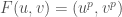
. It turns out that, in the group law on E, we have F^2 = [-p]. That is to say, F(F(u,v)) plus p copies of (u,v) is trivial.

I remember when I learned this trying to check it by hand, and being astonished at how out of reach the computation was. There are nice proofs using higher theory, but shouldn’t you just be able to write down an equation which had a pole at F(F(u,v)) and vanished to order p at (u,v)?

There is a nice way to check the prime 3 by hand. I’ll use \equiv for equivalence in the group law of E. Remember that the group law on E has -(u,v) \equiv (u,-v) and has (u_1,v_1)+(u_2,v_2)+(u_3,v_3) \equiv 0 whenever (u_1, v_1), (u_2, v_2) and (u_3, v_3) are collinear.

We first show that

\displaystyle{ F(u,v) \equiv (u-1, v) - (u+1, v) \quad (\dagger)}

Proof of (\dagger): We want to show that F(u,v), (u+1,-v) and (u-1,v) add up to zero in the group law of E. In other words, we want to show that these points are collinear. We just check:
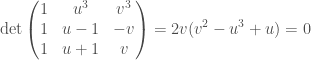
\displaystyle{ \det \begin{pmatrix} 1 & u^3 & v^3 \\ 1 & u-1 & -v \\ 1 & u+1 & v \end{pmatrix} =   2 v (v^2-u^3+u) = 0}

as desired. \square.

Use of (\dagger): Let (u_0, v_0) be a point on E. Applying F twice, we get

\displaystyle{ F^2(u_0,v_0) \equiv F \left( (u_0-1,v_0) - (u_0+1,v_0) \right)}

\displaystyle{  \equiv (u_0-2,v_0) - 2 (u_0,v_0) + (u_0+2,v_0)}.

Now, the horizontal line v=v_0 crosses E at three points: (u_0, v_0), (u_0-2, v_0) and (u_0+2, v_0). (Of course, u_0 -2 =u_0+1, since we are in characteristic three.) So (u_0-2, v_0) + (u_0, v_0) + (u_0+1, v_0)  \equiv 0 and we have

\displaystyle{F^2(u_0, v_0) \equiv -3 (u_0, v_0)}

as desired. \square.

I was reminded of this last year when Jared Weinstein visited Michigan and told me a stronger statement: In the Jacobian of y^2 = x^p-x, we have F^2 = [(-1)^{(p-1)/2} p], where F is once again the automorphism F(x,y) = (x^p, y^p).

Let me first note why this is related to the discussion of the elliptic curve above. (Please don’t run away just because that sentence contained the word Jacobian! It’s really a very concrete thing. I’ll explain more below.) Letting C be the curve y^2 = x^p-x, and letting p be 3 \mod 4, we have a map C \to E sending (x,y) \mapsto (y x^{(p-3)/4}, x^{(p-1)/2}), and this map commutes with F. I’m going to gloss over why checking F^2 = [(-1)^{(p-1)/2} p] on C will also check it on E, because I want to get on to playing with the curve C, but it does.

So, after talking to Jared, I was really curious why F^2 acted so nicely on the Jacobian of C. There are some nice conceptual proofs but, again, I wanted to actually see it. Now I do.

Continue reading

Rationality of the zeta function mod p

Here’s a neat argument about counting points that you could present at the end of a second course in number theory. I’m sure it’s not original, but, hey, that’s what blogs are for!

Let X be a smooth hypersurface in \mathbb{P}^{n}, over the field \mathbb{F}_p with p elements. The Weil conjectures are conjectures about the number of points of X over \mathbb{F}_{p^k}. Specifically, they say that there should be some matrix A such that

\displaystyle{ \# X(\mathbb{F}_{p^k}) = 1+p^k+p^{2k} + \cdots + p^{(n-1)k} + (-1)^{n-1} \mathrm{Tr} (A^k),}

and that the eigenvalues of A should be algebraic integers of norm p^{(n-1)/2}.
Here I am using the Lefschetz hyperplane theorem to know what H_{et}^i(X) is for i \neq n-1.

This is, of course, a famously hard theorem. The claim about the eigenvalues is the hardest part, but simply the existence of a matrix for which this formula holds is already quite hard; the first proof was due to Dwork.

What I am going to show you is that there is a much easier proof of the above formula modulo p; a proof of the sort that could be appear in Ireland and Rosen. Many of the terms above disappear mod p, so our goal is just to show that there is some matrix B such that

\displaystyle{ \# X(\mathbb{F}_{p^k}) \equiv 1 + (-1)^{n-1} \mathrm{Tr} (B^k) \mod p.}

Continue reading

The Weil Conjectures: The approach via the Standard Conjectures

The aim of this post is to outline a strategy for proving the Weil conjectures, proposed by Grothendieck and others. This strategy is incomplete; at various stages, we will need to assume conjectures which are still open today.

Our aim is to prove:

Theorem:
Let X be a smooth projective variety, over a field of any characteristic. Let H^* be a “reasonable” cohomology theory. Let \omega \in H^2(X) be the hyperplane class for a projective embedding of X. Let F be an automorphism of X, such that F^* \omega = q \omega. Then the eigenvalues of F^*: H^r(X) \to H^r(X) are algebraic numbers and, when interpreted as elements of \mathbb{C}, have norm q^{r/2}.

In previous posts, we gave for a proof in characteristic zero and a proof in the case that X is a curve. I also explained why I need to say how I am embedding these eigenvalues into \mathbb{C}. Our proof requires all the ideas of these previous posts, plus some new ones.
Continue reading

The Weil conjectures : Curves

Our goal for today is to prove the following theorem:

Theorem 1: Let X be a projective algebraic curve of genus g and F an endomorphism of degree q. Let H^* be a reasonable cohomology theory. Then the action of F^* on X has eigenvalues which are algebraic integers, with norm q^{1/2}.

For those who know the term, “reasonable cohomology theory” means “Weil cohomology theory”.

The consequence of this theorem, which does not mention cohomology, is

Theorem 2: Let X be a projective algebraic curve of genus g and F an endomorphism of degree q. Then there are algebraic integers \alpha_1, \alpha_2, …, \alpha_{2g} with norm q^{1/2} such that

\displaystyle{  \# \mathrm{Fix}(F^k) = q^k - \sum \alpha_i^k +1 }.

In a previous post, we established this in characteristic zero, by putting a positive definite hermitian structure on H^1(X, \mathbb{C}) such that q^{-1/2} F^* became unitary. But, as I discussed last time, we can’t define H^1(X, \mathbb{C}) when X has characteristic p. Instead, H^1(X) will be defined over some other field of characteristic zero, like \mathbb{Q}_{\ell}. We will therefore need to know that the eigenvalues of F are algebraic integers before we can even make sense of the statement that they have norm q^{1/2}.

It is possible to take the proof I present here and strip it down to its bare essentials, to give a proof of Theorem 2 which doesn’t even mention cohomology. See Hartshorne Exercise V.1.10. I am going to do the opposite; I will go slowly and focus on what each step is proving about H^1(X). The essential argument here is Weil’s, although I have modernized the presentation.

Continue reading

Characteristic zero analogues of the Weil conjectures: higher dimension

In our previous post, we proved

Theorem Let X be a smooth projective curve over \mathbb{C} and F an endomorphism of degree q > 0. The eigenvalues of F on H^1(X) have norm q^{1/2}.

Today, we would like to generalize this to varieties of higher dimension. The obvious guess is

Nontheorem Let X be a smooth projective variety, over \mathbb{C}, of dimension d. Let F be an endomorphism of X of degree q^d. The eigenvalues of F on H^r(X) have norm q^{r/2}.

This is not a theorem! I believe it is Serre who first figured out how to fix and prove this result. That is the topic of today’s post.
Continue reading

Characteristic zero analogues of the Weil conjectures: Curves

The quest to prove the Weil conjectures drove algebraic geometry throughout the middle of the twentieth century. It was understood very early that a proof should involve creating a theory of cohomology for varieties in characteristic p. This theory, known as étale cohomology, was developed by Grothendieck and his collaborators. Near the end, there was a period where étale cohomology was established but the hardest of the conjectures, the Riemann hypothesis, was not proved. Several mathematicians* proposed a path which would require proving results that were new even in the complex setting; results now known as the standard conjectures. That route was not taken; instead, Deligne found a different proof with its own insights and innovations.

This is the first of a series of posts sketching how the route through the standard conjectures would have gone. There is of course nothing original here; the usual sources are Kleiman, Grothendieck and Serre. I will try to write in a very classical way; I won’t even leave characteristic zero for the first two posts. And there will be tensor categories before the end!

In today’s post, we will prove the following theorem.

Theorem 1 Let X be a smooth projective curve over \mathbb{C} and F an algebraic endomorphism of degree q > 0. The eigenvalues of F on H^1(X) obey |\alpha|=q^{1/2}.

Continue reading

Christol’s theorem and the Cartier operator

Let’s suppose that we want to compute 2^n \mod p, and we have already been given n written out in base p as n = \sum n_i p^i. Here p is a small prime and we want to do this conversation repeatedly for many n‘s.

Remember that 2^p \equiv 2 \mod p and thus 2^n \equiv 2^{n_0+n_1 p + n_2 p^2 + \cdots + n_{\ell} p^{\ell}} \equiv 2^{n_0} 2^{n_1} \cdots 2^{n_{\ell}}  \mod p. So, start with 1, multiply it by 2^{n_0}, then by 2^{n_1}, then by 2^{n_2} and so forth. When you get to the end, read off 2^n.

We can precompute the effect on \mathbb{F}_p of multiplying by 2^k, for 0 \leq k \leq p-1. Then we can compute 2^n just by scanning across the base p representation of n and applying these precomputed maps to the finite set \mathbb{F}_p.

The precise way to say that this is a simple, one-pass, process is that it is a computation which can be done by a finite-state automaton. Here is the definition: let I, S and O be finite sets (input, states and output), and s \in S (the start). For each i \in I, let A(i) be a map S \to S. We also have a map r:S \to O (readout). Given a string (i_0, i_1, \ldots, i_{\ell}) in I^{\ell}, we compute r( A(i_{\ell}) \circ \cdots A(i_1) \circ A(i_0) (s)). So our input is a string of characters from I, and our output is in O.

We can say that our example above shows that (n_{\ell}, \ldots, n_1, n_0) \mapsto 2^{\sum n_i p^i} \mod p is computable by a finite-state automaton. (In our example, the sets I, S and O all have cardinality p, but I do not want to identify them.)

This is a special case of an amazing result of Christol et al: Let f_n be a sequence of elements of \mathbb{F}_p. Then (n_{\ell}, \ldots, n_1, n_0) \mapsto f_{\sum n_i p^i} can be computed by a finite-state automaton if and only if the generating function \sum f_n x^n is algebraic over \mathbb{F}_p(x)!

We have just explained the case \sum f_n x^n = 1/(1-2x). The reader might enjoy working out the cases 1/(1-x-x^2) (the Fibonacci numbers) and (1 - \sqrt{1-4x})/2x (the Catalans).

In this post, I will use Christol’s theorem as an excuse to promote the Cartier operator, an amazing tool for working with differential forms in characteristic p.

Continue reading

More F_un

Incidentally, I hope you’ve all been reading F_un mathematics. Even if you aren’t all that interested in the field with one element, it’s a beautifully designed site and might give you some ideas about pushing Web 2.0 in mathematics a bit further than just blogs. While I like our blog, with all its messy diversity (as my collaborators can tell you, messy diversity is a core component of my mathematical style), F_un mathematics has a much more organized focused feel, which I think maybe more promising for getting actual mathematics done. I also think the division of the posts into “outreach,” “undergraduate,” “graduate,” and “research” has some interesting potential and sort of makes me feel like we should be doing a better job of indicating the background level for our post.

Uniform Position in Characteristic p

Let X be an irreducible degree d curve in \mathbb{C} \mathbb{P}^r. Some hyperplanes will be tangent to X, or pass through singularities of X, or even perhaps contain X. But most hyperplanes won’t do any of these things. Let U be the space of hyperplanes which do not exhibit any of these bad behaviors; these hyperplanes are said to be transverse to X. Every hyperplane H in U meets X in d points. As we move H through U, these d points move around X. If H navigates a loop in U, before returning to itself, then these d points are permuted. Last week, in his class on Algebraic Curves, Joe Harris proved the following theorem.

The Uniform Position Principle: Let G and H be two hyperplanes in U, with G \cap X = \{ x_1, \ldots, x_d \} and H \cap X = \{ y_1, \ldots, y_d \}. Then, for any permutation \sigma \in S_d, there is a path from G to H within U such that traveling along this path takes x_i to y_{\sigma(i)}.

In this proof, it was crucial that we were working with a field of characteristic zero. The key lemma was that there was a little loop in U such that traveling around that loop swapped exactly two points. The proof, in sketch, is to find a hyperplane H_0 which is not transverse to U, but just barely; so that H_0 is tangent to X at one point and meets X transversely at d-2 other points. If we then wiggle H_0 in a little disc, then the tangency point of X and H_0 will separate into two distinct points, while the other d-2 points will wiggle around a little. The boundary of that disc will be a loop in U and (exercise!) as you travel around that loop, the two perturbations of the tangency point switch with each other.

In characteristic p, there are curves for which there are no such tangent planes H_0. As I’ll show you soon, there exist curves X where every single point x \in X is a flex, meaning that the tangent line to X at x touches X with degree \geq 3. So the proof falls apart. We got into a discussion in Harris’ class about whether the result also falls apart. I’ve done some computations and the answer is “yes”. Moreover, the monodromy groups we get are very pretty. Continue reading