Our goal for today is to prove the following theorem:
Theorem 1: Let  be a projective algebraic curve of genus
  and
and  an endomorphism of degree
  . Let
. Let  be a reasonable cohomology theory. Then the action of
  on has eigenvalues which are algebraic integers, with norm
  .
.
For those who know the term, “reasonable cohomology theory” means “Weil cohomology theory”.
The consequence of this theorem, which does not mention cohomology, is
Theorem 2: Let be a projective algebraic curve of genus and an endomorphism of degree . Then there are algebraic integers  ,
,  , …,
, …,  with norm such that
 .
.
In a previous post, we established this in characteristic zero, by putting a positive definite hermitian structure on  such that
  became unitary. But, as I discussed last time, we can’t define when has characteristic
  . Instead,
  will be defined over some other field of characteristic zero, like
  . We will therefore need to know that the eigenvalues of are algebraic integers before we can even make sense of the statement that they have norm .
It is possible to take the proof I present here and strip it down to its bare essentials, to give a proof of Theorem 2 which doesn’t even mention cohomology. See Hartshorne Exercise V.1.10. I am going to do the opposite; I will go slowly and focus on what each step is proving about . The essential argument here is Weil’s, although I have modernized the presentation.
The ring 
We define a ring as follows: The elements of the ring are formal sums of curves in  , modulo the relation that
 ![[C] = [C']](https://s0.wp.com/latex.php?latex=%5BC%5D+%3D+%5BC%27%5D&bg=ffffff&fg=444444&s=0&c=20201002) if the curves
if the curves  and
and  have the same class in
  . We multiply as follows:
![[C] \bullet [C'] = (\pi_{13})_* ( \pi_{12}^* [C] \cdot \pi_{23}^* [C']),](https://s0.wp.com/latex.php?latex=%5BC%5D+%5Cbullet+%5BC%27%5D+%3D+%28%5Cpi_%7B13%7D%29_%2A+%28++%5Cpi_%7B12%7D%5E%2A+%5BC%5D+%5Ccdot+%5Cpi_%7B23%7D%5E%2A+%5BC%27%5D%29%2C&bg=ffffff&fg=444444&s=0&c=20201002)
where the  are the three projections
  .
.
Fans of This Week’s Finds will recognize this as a slight variant of the category of spans.
Notice that the diagonal,  , of , is the multiplicative identity of .
The cohomology groups  are modules for by
![[C] \bullet \alpha = (\pi_1)_* ( [C] \cdot \pi_2^* \alpha)](https://s0.wp.com/latex.php?latex=%5BC%5D+%5Cbullet+%5Calpha+%3D+%28%5Cpi_1%29_%2A+%28+%5BC%5D+%5Ccdot+%5Cpi_2%5E%2A+%5Calpha%29&bg=ffffff&fg=444444&s=0&c=20201002) . In particular, if
. In particular, if  is an endomorphism of , and
  is the graph of , then
 ![[\Gamma]](https://s0.wp.com/latex.php?latex=%5B%5CGamma%5D&bg=ffffff&fg=444444&s=0&c=20201002) acts on by
acts on by  .
.
Let  and
and  be the classes in of
  and
and  . Then and are orthogonal idempotents. Define
  , so
, so  is also idempotent. Then
  acts by
  on and by
  on every other
  .
.
Since the are orthogonal idempotents, we have  . You can compute that
  and
and  , so all the interest is in
  . We’ll write
  for ; so is a module.
The involution 
We define an involution ![[C] \mapsto [C]^{\dagger}](https://s0.wp.com/latex.php?latex=%5BC%5D+%5Cmapsto+%5BC%5D%5E%7B%5Cdagger%7D&bg=ffffff&fg=444444&s=0&c=20201002) of which sends a curve to the curve
of which sends a curve to the curve  obtained by switching the two factors of . You can check that sends to itself.
In our previous proof, we put a positive definite Hermitian structure on .
Exercise: If is a curve over  , and
, and  is in , then the actions of and
  on are adjoint.
There is a point that confused me when I first learned this stuff. We never mention complex conjugation in the definition of , so how can we get the Hermitian conjugate? The answer is simple: the maps coming from the action of are defined over  (in fact,
  ). So is adjoint to with respect to both the natural skew-symmetric pairing on , and with respect to its Hermitian complexification. This is just like how, for a real matrix, the transpose and the conjugate transpose are the same thing. The question of whether to think in terms of Hermitian or ordinary bilinear forms is somewhat of an aesthetic choice; perhaps at some later point I will defend my decision to use the Hermitian language.
Let  be the graph of , and let
  . Since is not a complex vector space, we cannot say that
  is unitary.
But there is a statement which still makes sense:
Exercise: We have  .
.
The linear form 
Finally, define a linear form  by
by  , using the intersection product in
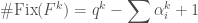
  . By the Lefschetz trace formula, we have


Note that the left hand side is an integer, while the right hand side, a priori, need only lie in the coefficient ring of  . It is this ability to get an integer, rather than an element of , that will resolve our difficulties with coefficients.
In our previous proof, it was crucial that the Hermitian form on was positive definite. The corresponding result here is
Key Lemma: The -valued inner product  on is negative definite.
If is defined over , this follows from the positive definiteness of the Hermitian form. (We pick up the minus sign because  is
is  for in .) But the Key Lemma makes sense over any field because, regardless of what ring our cohomology theory takes coefficients in, the ring is still a -module, and the pairing is still -valued.
Proof of the main theorem from the key lemma
 acts by zero on
  and
and  . So
. So  , where
  are the eigenvalues of acting on . Since
  is always an integer, we deduce that
  is an integer for every
  . This immediately implies that the are algebraic numbers and, working a bit harder (exercise!) that they are algebraic integers.
The Key Lemma tells us that  is negative definite. So, by Cauchy-Schwartz,
 .
.
In other words,

and
 .
.
Similar arguments show that  for all . From this is follows that
  . Applying similar arguments to
  , we can also deduce that
  , so
, so  .
.
Proof of the key lemma
We consider the form  on all of , instead of just . Then
  has block form

where the middle block is the pairing on . So, to prove that is negative definite on , it is enough to prove that has signature of the form  on . For a proof of this fact, see Hartshorne Theorem V.1.9 and Remark V.1.9.1.
Connection to the Hodge Index Theorem
When our ground field is , there is a nice proof that has signature on , using the Hodge index theorem. We’ll be reusing notation from my previous post, so you might want to follow that link to refresh your memory.
By definition,  and, in fact, lies in
  . Reusing our notation from an earlier post,
  . But
. But  , so
, so  is one dimensional. Then the Hodge index theorem says that is positive definite on
  and negative definite on the orthogonal space
  . We see that has signature
  on
on  . Its signature on the subspace must thus be of the form either or
  ; it is easy to check that it is the former.
The fact that has signature on can thus be thought of as a shadow of the Hodge index theorem, which remains even when our cohomology theory takes coefficients in an exotic ring. We will return to this point next time, when we tackle Grothendieck’s Standard Conjectures.

2 thoughts on “The Weil conjectures : Curves”
Comments are closed.