Here’s a basic example that comes up if you work with elliptic curves: Let  be a prime which is
  . Let
. Let  be the elliptic curve
  over a field of characteristic . Then has an endomorphism
  . It turns out that, in the group law on , we have
 ![F^2 = [-p]](https://s0.wp.com/latex.php?latex=F%5E2+%3D+%5B-p%5D&bg=ffffff&fg=444444&s=0&c=20201002) . That is to say,
. That is to say,  plus copies of
  is trivial.
I remember when I learned this trying to check it by hand, and being astonished at how out of reach the computation was. There are nice proofs using higher theory, but shouldn’t you just be able to write down an equation which had a pole at and vanished to order at ?
There is a nice way to check the prime  by hand. I’ll use
  for equivalence in the group law of . Remember that the group law on has
  and has
  whenever
  ,
,  and
and  are collinear.
We first show that

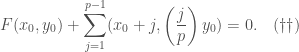
Proof of  : We want to show that
  ,
,  and
and  add up to zero in the group law of . In other words, we want to show that these points are collinear. We just check:
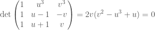
as desired.  .
.
Use of : Let  be a point on . Applying
  twice, we get

 .
.
Now, the horizontal line  crosses at three points: ,
  and
and  . (Of course,
  , since we are in characteristic three.) So
  and we have

as desired. .
I was reminded of this last year when Jared Weinstein visited Michigan and told me a stronger statement: In the Jacobian of  , we have
 ![F^2 = [(-1)^{(p-1)/2} p]](https://s0.wp.com/latex.php?latex=F%5E2+%3D+%5B%28-1%29%5E%7B%28p-1%29%2F2%7D+p%5D&bg=ffffff&fg=444444&s=0&c=20201002) , where is once again the automorphism
, where is once again the automorphism 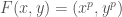 .
.
Let me first note why this is related to the discussion of the elliptic curve above. (Please don’t run away just because that sentence contained the word Jacobian! It’s really a very concrete thing. I’ll explain more below.) Letting  be the curve , and letting be , we have a map
  sending
  , and this map commutes with . I’m going to gloss over why checking on will also check it on , because I want to get on to playing with the curve , but it does.
So, after talking to Jared, I was really curious why  acted so nicely on the Jacobian of . There are some nice conceptual proofs but, again, I wanted to actually see it. Now I do.
Let be any odd prime. Let be the curve  , over a field of characteristic . We’ll be working in the Jacobian of . This is a group
  , generated by the points of , and subject to the relation that, if there is a polynomial
  vanishing precisely at the points
  ,
,  , …,
, …,  , then
  . If you’ve seen this theory laid out for projective curves, then you use rational functions rather than polynomials, and you have to keep track of poles as well as zeroes. Because I’m using the affine curve , I get to just work with polynomials and their zeroes.
When we run this construction for a curve of the form  , then the elements of the group are just the points on the curve, plus the additive identity. Let’s see why:
  , as these are the two points on the line
  , so we don’t need formal inverses. And for any two points and with
  , the line through these points will meet the curve once more, say at
  , so we have
  . We can repeatedly use this trick to reduce sums of many points to sums of fewer points.
I am now asking you to consider , which (except when  ) is not of the form
. This means that not every element of will be equivalent to a single point of the curve . Other than that, the theory really isn’t harder.
The curve has an endomorphism , just as before. And, just as before, what we are going to be showing is that  as endomorphisms of the group . In particular, when
  , we have
  .
.
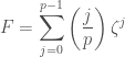
The key identity
We’re going to figure out how to generalize equation for all primes. The equation we want is
 .
.
Here  is the quadratic residue symbol: it equals
  if
if  is a quadratic residue modulo ; it equals
  if is a non-QR and
  if
if  .
.
Just as in the case, we’ll want to rewrite this to have fewer minus signs. For any  on , the vertical line meets at two points: and
  . So
. So 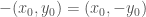 . So we can rewrite our desired equation as
 .
.
So we need to find a polynomial which passes through the points  . Set
. Set
 .
.
Since  , the polynomial
  will pass through all of the points . Where else does
  meet ?
Well, if then  . Plugging this into the equation for , we have

or
 .
.
This is a degree polynomial in  . We already know
  of the roots — they are at
  for a nonzero element of
  .
.
Equation  has leading term
  , and constant term
  . So we can conclude that the product of the roots of is
  . We have
  . So the last root of is at
  . A little more thought shows that the intersection of with is at
  , not
, not  .
.
So we have found a polynomial which vanishes precisely at the points  and
and  , and we have proved equation
  .
.
Why we’ve won
Let  be the automorphism
  of the curve . Clearly,
  . A little less obviously, I claim that
  in the endomorphism ring of the group . In other words, I am claiming that, for any on , we have

This is because the points  are precisely the intersections of with the horizontal line
  .
.
So is a module for the ring ![\mathbb{Z}[\zeta]/(1+\zeta+\cdots+\zeta^{p-1})](https://s0.wp.com/latex.php?latex=%5Cmathbb%7BZ%7D%5B%5Czeta%5D%2F%281%2B%5Czeta%2B%5Ccdots%2B%5Czeta%5E%7Bp-1%7D%29&bg=ffffff&fg=444444&s=0&c=20201002) . This is better known as the ring of cyclotomic integers. And identity tells us that
. This is better known as the ring of cyclotomic integers. And identity tells us that
in the ring  .
.
The right hand side of the above equation is a very famous element of  : The Gauss sum. And it’s most famous property is that — exactly what we wanted to show.
Let’s review why the Gauss sum has the desired square.

.
Group together terms with the power of to get
 .
.
If  , then
  takes on every value in once, except that it misses . If
  , then takes on the value over and over, times in total. Using
  , our sum is

as desired.
What I want to emphasize is that every equality of this proof corresponds to writing down a rational function on with the corresponding poles and zeroes. For example, the second to last equality above replaced  by . There is a corresponding rational function which has zeroes at
 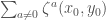 and has a pole at : Namely,
  . It would be painful, but completely doable, to actually use this proof to write down a rational function on with a zero at , and a -fold pole at
  . In fact, I cheated a bit in the beginning of this post. I didn’t just cleverly guess the formula ; I instead wrote down and plugged in .
Descending the resulting rational function to the curve  would probably leave an unmotivated mess. I understand how to do it: You need to look at the rational function of
  and rewrite it in the variables ; Galois theory guarantees that you will succeed. But I suspect the result would be unenlightening.
So, finally, I understand why  without going through the theory of supersingular curves, or the Weil bounds, or anything deeper than Gauss sums. Hope you enjoyed!

You have a little mixup in notation at the beginning: you define E as u^2=v^3-v, but then you prove things about v^2=u^3-u.
Looking forward to reading the rest of this!
(this is Alison Miller).
Thanks Allison!
Jared also e-mailed and mentioned that a similar trick should work for and indeed it does. For
  , let
, let  be the automorphism
  . Let
. Let  be
be  . Then looking at the intersections of
 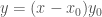 with
with  shows that
 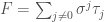 . The group generated by the
  ‘s is isomorphic to
  ; the ring of endomorphisms generated by
  and the
  is isomorphic to
By mapping and
and  to various nontrivial
  -th and
  -st roots of unity, the element
  get’s sent to all of the various Gauss sums. I haven’t checked this carefully, but I believe the right statement should be that each of the
  nontrivial Gauss sums appears once in the cohomology of
  .
.