I’m teaching a graduate course in symplectic geometry and GIT this semester, and am going to try to produce some posts related to lectures I’m giving there. Hopefully, this will help me think things through and put some new exposition out there on the internet.
So, obviously, the first question is “what is a symplectic manifold?” Now, wikipedia will tell you it’s a manifold equipped with a non-degenerate closed 2-form. Certainly that’s right, but it doesn’t tell a novice in symplectic geometry much. Why think about such a structure?
So let me try to put a different spin on this. This isn’t all that new of a spin (in fact, Henry Cohn wrote almost exactly the same thing here), but I don’t know of anywhere symplectic manifolds are really presented like this: I want to think of a symplectic manifold as a space where one can do a particular flavor of classical mechanics. I’m going to define a mathematical object called a phase space. This is supposed to be a set of observable facts about a physical system (a “phase”); each point might represent a specific position and specific momentum, or it might be something coarser. Informally, we want that if we specify an energy function which only depends on the phase, then we can tell how the phase evolves with time, and this evolution is “reasonable.” More formally a phase space is a manifold 
- If
is a smooth compactly supported function, then there is a time evolution
such that
. Physically, we think of this as the energy function specifying how the system evolves over time.
- Conservation of energy:
.
- No conserved quantities: for any two points
and
, there is a chain of energy functions and times
such that applying the time evolution for the
‘s in order for
goes from
- Linearity under superposition: the flow
is the exponential of a vector field
, and we have that
and $X_{cf}=cX_f$ for all constants $c$.
- Equilibrium: if
, then
for all
.
- The assignment from energy functions to flows is equivariant under any of the flows:
.
All of these are hopefully intuitive properties for a physically system to have.
For example, if we let 


This gives a rule for obtaining 
Now, I hope you’ve all guessed what the coming theorem is:
Theorem. A phase space is the same thing as a symplectic manifold.
So, given a phase space, how does one find the symplectic structure? Well, by the equilibrium condition, the vector $X_f$ at a point depends only on $df$: if 


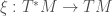
Of course, an isomorphism between a vector bundle and its dual can be thought of as an element of its tensor square 


That is, if we let 


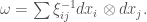
I’d like to show that this is a 2-form, that is, that 
So, by conservation of energy applied to the function 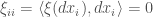


We’re almost to a symplectic manifold. We have a non-degenerate 2-form, we just need to know why its closed. Conveniently, we have one axiom we haven’t used: the equivariance of the assignment from energies to flows under the flows themselves. We can how restate this in terms of

By definition, we have that 

which is the same as saying that 
Hooray! That finishes the proof one direction: the proof of the other direction can be found (in scattered pieces) in any text on symplectic geometry. The vector field 


This ends our first installment; I’ll continue as I come across bits of exposition that I think actually add to the exposition in Cannas da Silva.

Henry Cohn discussed similar ideas here.
“No conserved quantities” is a cute name for the condition that there’s only one symplectic leaf, but I’m a little bothered by it. I would have thought a “conserved quantity” was, say, a Casimir, and there are plenty of Poisson manifolds with trivial Poisson center. I do agree that “no conserved quantities” is a reasonable physical axioms: the only way we set up experiments is by manipulating the energy functions involved, and the axiom is that we can in fact prepare any state from any other.
This depends on how you interpret “quantity;” after all, if there is more than one symplectic leaf (and the space is connected), one of the leaves is lower dimensional, and there is some function that is constant on that leaf. From the perspective someone living on the smaller leaf, that observable is conserved.
Qiaochu- Good catch. Great minds think alike, I guess.
If I remember well symplectic manifolds and geometry were introduced by Arnold (Mathematical Methods of Classical Mechanics) and since the (only) reason to impose closedness of the symplectic form is as a slick formulation of “invariant under hamiltonian phase flows” we have the following interesting historical situation.
Arnold was very critical of Bourbaki but in his book he states the definition of a symplectic manifold, including closedness of $\omega$ and then proves a “Theorem: The form… is an integral invariant of a hamiltonian phase flow.”.
But nowadays, accustomed as we are now to wikipedia and mathoverflow intuitive explanations, we know this is misleading, the real theorem is that we can characterize/axiomatize symplectic forms (i.e. those yielding invariants under hamiltonian flows, in particular the volume form) as closed forms.
So history has produced this educationally awkward situation: the presentations based on time/flow-invariance which are (it seems to me) absolutely necessary to make any sense of the “closed form” condition are not standard.
(I am no expert and may be wrong. I apologize if I am and please correct me.)
There is of course another physical explanation: (Pre-)Symplectic manifolds arise from variational principles.Since most of classical physics can be described by such a principle it is natural to consider symplectic manifolds. Along this road one will immediatly encounter moment maps and so on.